Getting Started¶

The Langmuir library contains a collection of functions that compute the current collected by a conductor immersed in a plasma according to various models (characteristics). These functions take as arguments the probe geometry, for instance Sphere, and a plasma, where a plasma may consist of one or more Species.

As an example, consider a spherical Langmuir probe of radius $r=1\,\mathrm{mm}$ immersed in a plasma with an electron density of $n=10^{11}\,\mathrm{m^{-3}}$ and an electron temperature of $T=1000\,\mathrm{K}$ . The electron current collected by this probe when it has a voltage of $V=4.5\,\mathrm{V}$ with respect to the background plasma is computed according to orbital motion-limited (OML) theory as follows:

>>> OML_current(Sphere(r=1e-3), Electron(n=1e11, T=1000), V=4.5)
-5.262656728335636e-07

Let’s consider a more complete example. Below we compare the current-voltage characteristics predicted by the OML theory and the finite-length (FL) model for a cylindrical probe with an ideal guard on one end.

from langmuir import *
import numpy as np
import matplotlib.pyplot as plt

plasma = [
    Electron(n=1e11, T=1000),
    Hydrogen(n=1e11, T=1000)
    ]

geometry = Cylinder(r=1e-3, l=60e-3, lguard=True)

V = np.linspace(-2, 2, 100)

I_OML = OML_current(geometry, plasma, V)
I_FL = finite_length_current(geometry, plasma, V)

plt.plot(V, -I_OML*1e6, label='OML')
plt.plot(V, -I_FL*1e6, label='FL')
plt.xlabel('V [V]')
plt.ylabel('I [uA]')
plt.legend()
plt.show()

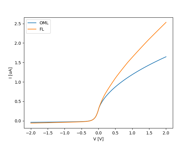
This example demonstrates that accounting for edge effects on a probe of finite length leads to a larger collected current. Also note that the characteristic correctly captures both the electron saturation, the electron retardation, and the ion saturation regions. Beware that the current collected by Langmuir probes (thus going into it) is usually negative. It is common practice, however, to invert it prior to plotting.